Are Autoencoders Fundamentally Denoisers?

The core idea behind Autoencoders is to bottleneck information flow so that the DNN is forced to prioritize what information to propagate to the next layer (by restricting the number of dimensions in the latent space). In this project, I explore how this can be a useful denoising tool.

Outline

This project generates thousands of synthetic signals (samples) of differnt frequencies, corrupts them with random noise and then trains an Autoencoder to recover the signal. I also experiment with different model depths and noise intensities to assess how well the base signal can be recovered. The broad outline is as follows:

1. Generating the Corrupted Signals
2. Defining the Model
3. Training the model to Denoise the Signal
4. Visualizing the Training
5. Visualizing the Recovered Signal

Synthetic Dataset Generation

To evaluate the denoising performance of different autoencoder architectures, we created a synthetic dataset by generating time-series samples based on random frequency sinusoidal functions. The generation process is broken down as follows:

• Base Signal Generation:

  The base signal, \( f(x) \), for each sample is generated using a combination of sine and cosine functions with randomized frequencies: \[ f(x) = \sin(f_1 \cdot x) + \cos(2 \cdot f_2 \cdot x) \] where:

  • \( f_1 \) and \( f_2 \) are random frequencies chosen uniformly within a specified range (e.g., between 0.5 and 2.5).
  • \( x \) represents time steps from 0 to \( 4\pi \) with a fixed interval, yielding a consistent sequence length for each sample.

  This approach produces a diverse dataset of base signals with varying frequencies, which introduces variability while maintaining a consistent signal form for analysis.

• Adding Noise to the Signal:

  To simulate noisy signals, we introduce varying levels of random white noise controlled by a parameter \( \alpha \). The noisy signal \( g(x) \) for each level of \( \alpha \) is generated as follows: \[ g(x) = (1 - \alpha) \cdot f(x) + \alpha \cdot \text{random_noise} \] where:

  • \( \alpha \) represents the noise level, ranging between 0 and 1. A lower \( \alpha \) corresponds to a cleaner signal, while a higher \( \alpha \) increases the noise.
  • random_noise is sampled from a standard normal distribution.

  For each value of \( \alpha \), a separate dataset is created, maintaining a constant base signal \( f(x) \) across different noise levels. This setup allows us to assess the denoising capability of each autoencoder configuration by comparing results on datasets with varying noise intensities.

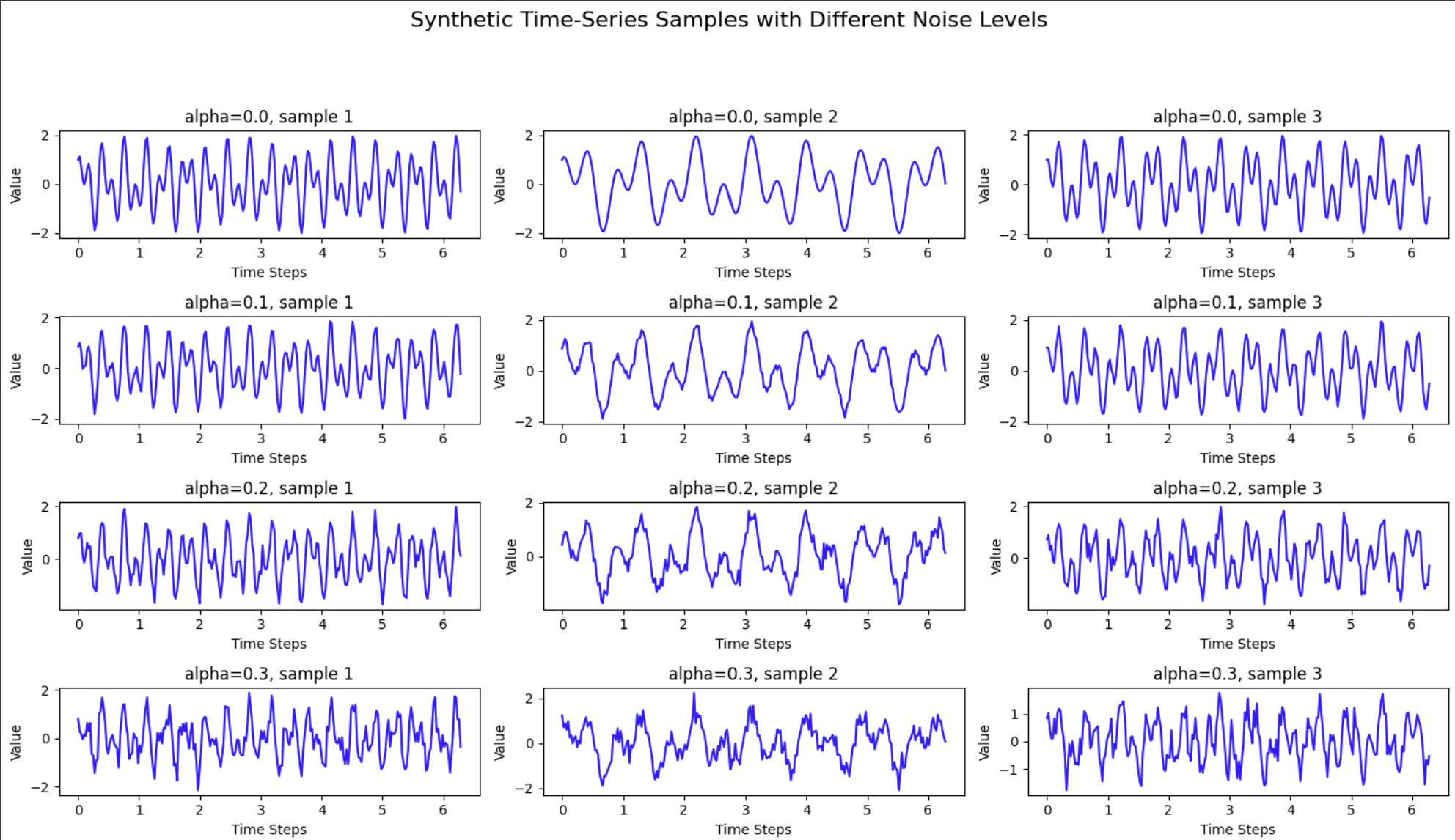
From top to bottom, the signal gets more noisy (denoted by the level of alpha). Each column represents an individual sample.

Autoencoder Model

The denoising model is an autoencoder architecture that leverages 1-dimensional convolutional layers to process 1-D time-series data. The model structure includes:

• 1-D Convolutional Downsampling (Encoder):

  The encoder consists of a sequence of 1-D convolutional layers that progressively downsample the input signal, extracting higher-level features while reducing spatial dimensions. The number of downsampling layers, \( d \), can be varied to control the model depth and capture progressively complex representations of the input signal.

• 1-D Convolutional Upsampling (Decoder):

  The decoder reconstructs the signal by progressively upsampling the encoded features using transposed 1-D convolution layers. The number of upsampling layers, \( u \), matches the encoder’s depth to produce an output with the same dimensionality as the input signal.

• Architecture Inspiration:

  This architecture is inspired by the U-Net model but modified to use 1-D convolutions for handling time-series data instead of 2-D convolutions used for image data. Unlike a traditional U-Net, the autoencoder we use here omits skip connections, which may be beneficial for complex structures but might be unnecessary for a relatively simple denoising task.

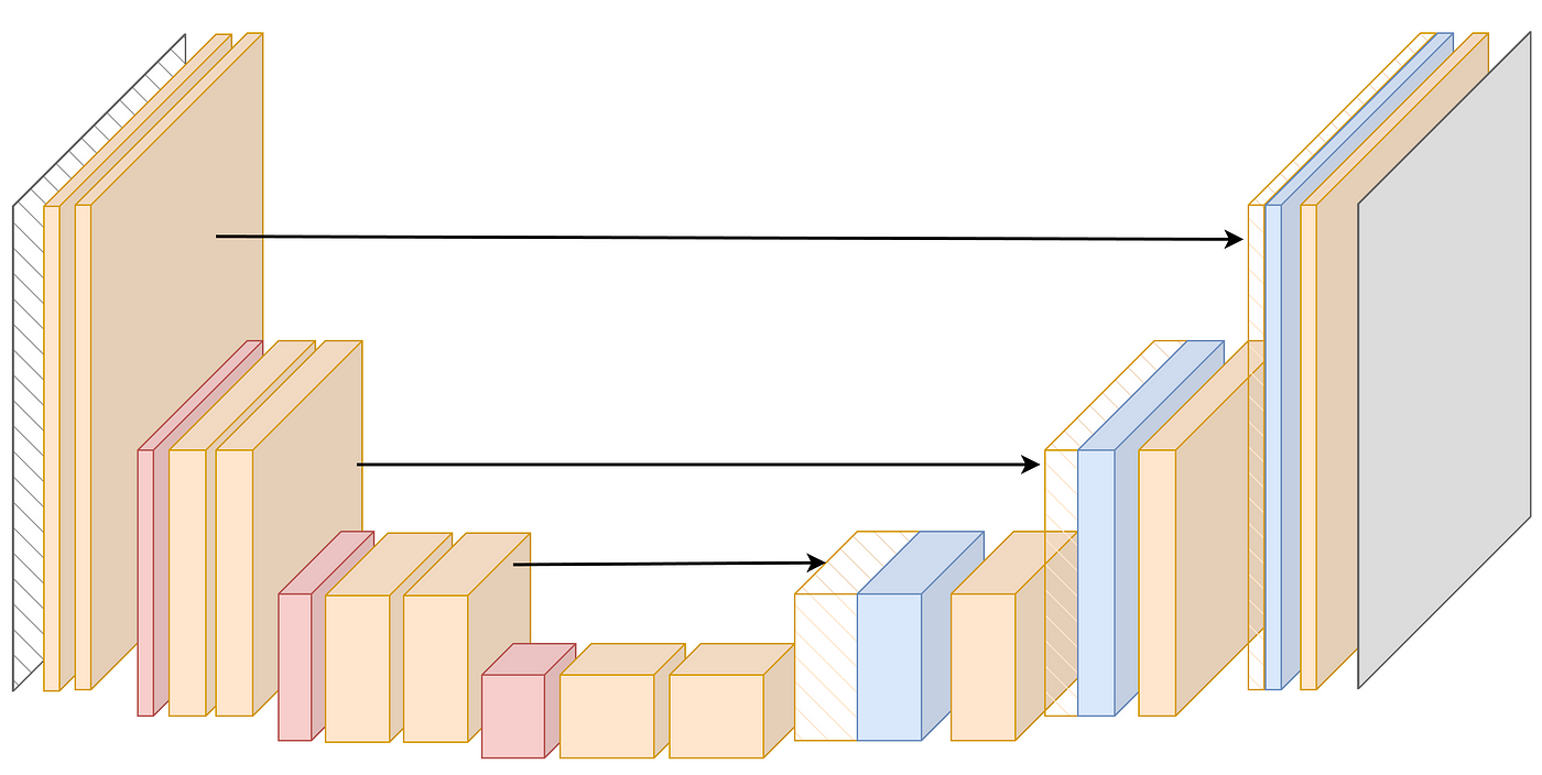
Source. U-NET Architecture. This project’s architecture is similar but doesnt have skip connections and uses 1-D convolution filters instead of the 2-D ones shown above.

Dataset Split

To train and evaluate each autoencoder variant effectively, we split the dataset into training and validation sets as follows:

• Training Set: 70% of the data for each noise level was used for training the model, allowing it to learn to denoise signals at varying intensities.
• Validation Set: 30% of the data was used for validation, which helped us monitor the model’s performance and detect overfitting as it trained.

This split ensures a robust evaluation by testing the model on unseen data from the same distribution as the training set.

Training Autoencoders of Different Depths

To study the impact of model depth on denoising performance, we trained autoencoders with different combinations of downsampling (d) and upsampling (u) layers. Each depth variant was trained across all datasets, allowing us to assess how well different model depths denoise signals with varying noise levels.

• Model Variants: Each model variant is defined by its depth, where \( d = u \), and we trained models with several configurations, such as \( (d, u) = (2, 2), (4, 4), (6, 6) \), and \( (8, 8) \).
• Training Process:
  • For each combination of depth and noise level, the model was trained independently. This led to a total of \( \text{number of depth configurations} \times \text{number of noise levels} \) models.
  • The loss was computed by taking the mean squared error (MSE) between the model’s output and the corresponding base signal for each sample, ensuring that the model learned to reconstruct the original signal.

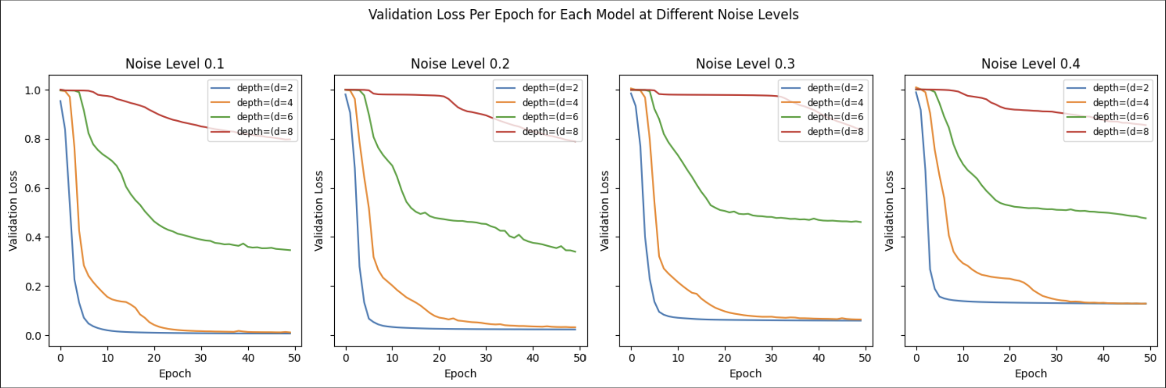
Validation loss across different noise levels. The deeper the model, the worse the denoising.

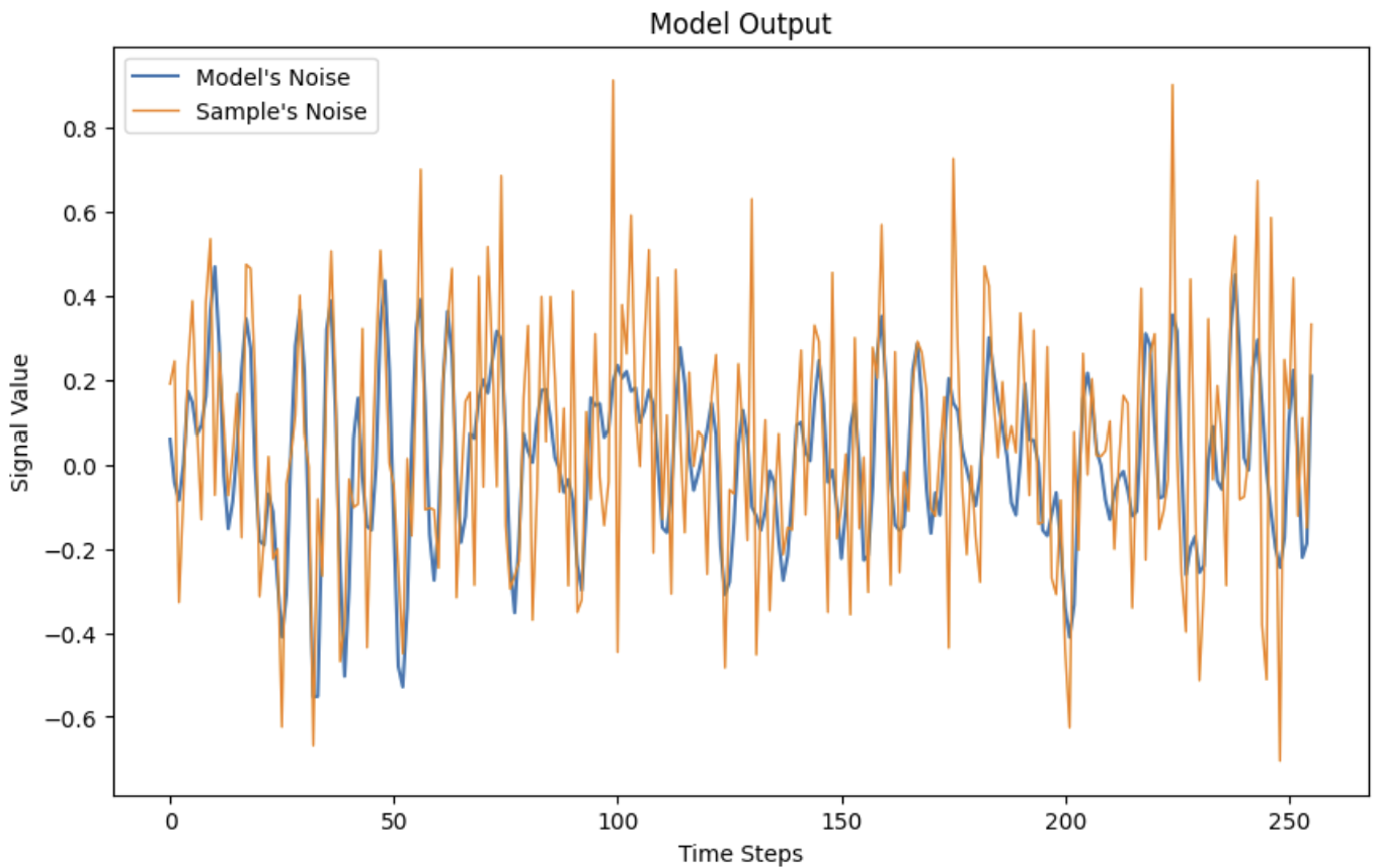
Plotting the noise in the model’s output (model output - base signal) and the corrupted sample (corrupted sample - base signal) to understand how much noise was removed by the model.

The trained models’ performance was compared by evaluating the validation loss for each depth configuration across different noise levels. This analysis helps to identify the optimal depth configuration that best generalizes across varying noise intensities, balancing complexity and denoising ability.

Conclusion

By using synthetic time-series data with controlled noise levels and training autoencoders of varying depths, this approach provides insights into how well different architectures perform in denoising tasks.

References

1. Google Colab for the Project.