Review: A Mathematical Framework for Transformer Circuits

This paper provides a mental model for reasoning about the internal workings of transformers and attention heads in deep neural networks. The insights here help understand and analyze the behaviors of large models.

General Notes

1. This paper offers a clear mental framework for thinking about transformers and attention heads, which is helpful for reasoning about large models.
2. Frequently, computations within transformers are restructured for efficiency, making the operations less interpretable. Therefore, it is possible to find multiple expressions for the same operation, which are typically mathematically equivalent but may differ in clarity.

Residual Stream

The residual stream is essential to understanding transformer architecture. It allows the model to bypass layers as needed, as it doesn’t require going through all layers. This is possible because every attention head and MLP layer simply adds its information back to the residual stream.

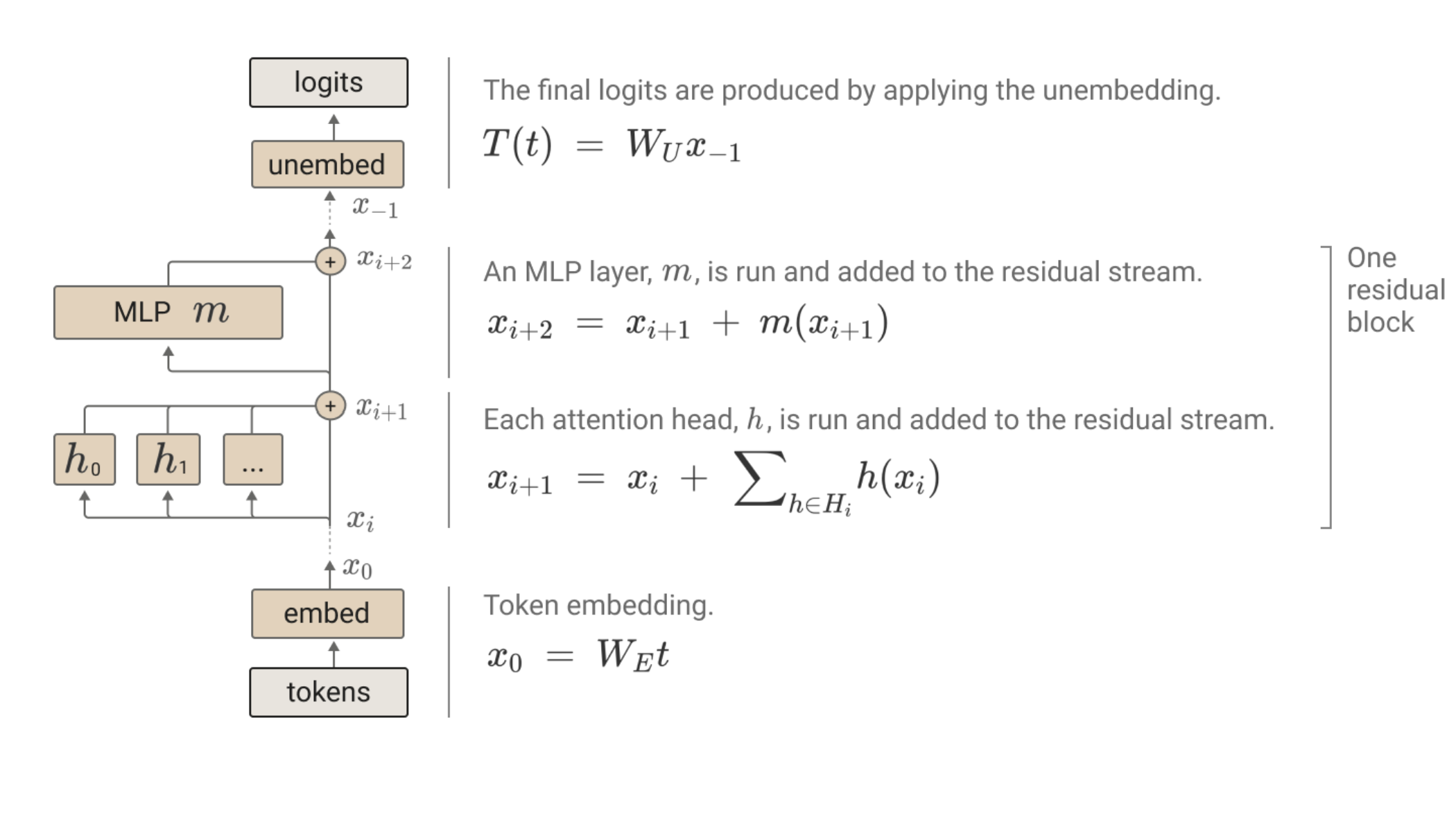Architecture: The center line (from embed to unembed) is the residual stream.

Each head reads from the entire residual stream (including both original tokens and the information added by previous heads) and outputs a vector, which is then added back to the residual stream. Every head operates on a subspace of the residual stream, allowing components to communicate by encoding information within specific subspaces. For instance, one attention head can write information to a particular subspace, which another head can then read. This functionality enables attention heads and MLPs to use the residual stream to share information effectively.

Often, individual heads appear to perform distinct, hypothesized functions that can be isolated and analyzed.

Superposition and Interference in the Residual Stream

The residual stream often encodes more features than there are dimensions, so these features are approximately orthogonal (dot products close to zero). When projecting the residual stream to a smaller space, some interference can occur since the features are not fully orthogonal. However, since features are typically sparsely activated during training, this interference does not usually hinder model performance. If features occurred frequently together, interference would become more problematic.

Attention Heads

1. An attention layer consists of multiple attention heads working independently and in parallel, with each head focusing on a subspace of the residual stream across all tokens in a sequence.

2. Each token in the sequence plays two roles: (i) A source of information for other tokens and (ii) A destination of information from other tokens. This can be summarized as below.

   

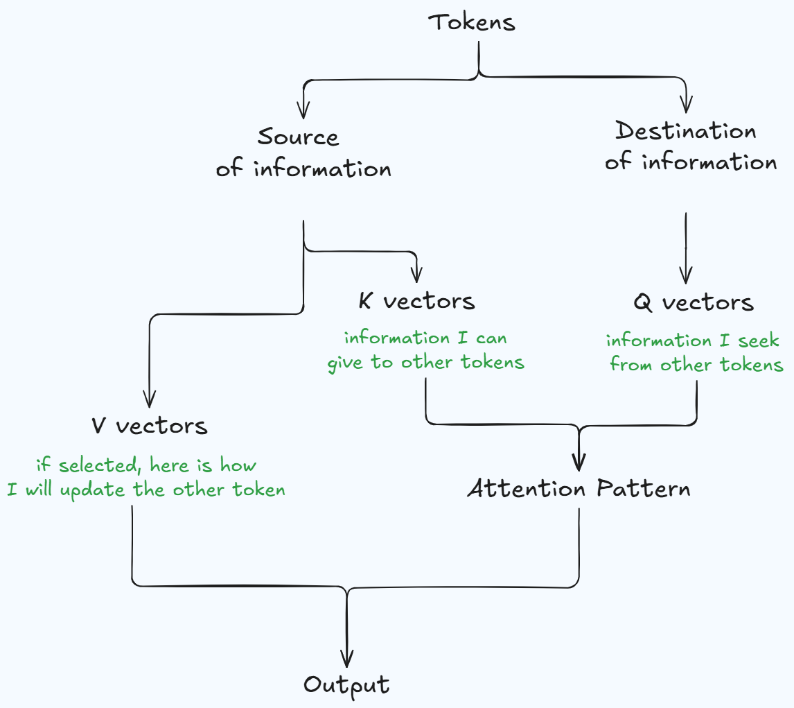
3. Within a single head: for each token, the head learns a probability distribution over that token and all previous tokens. This probability distribution represents the relative importance (context) of each previous token for the current token. The weights are normalized using softmax, ensuring each row sums to 1.
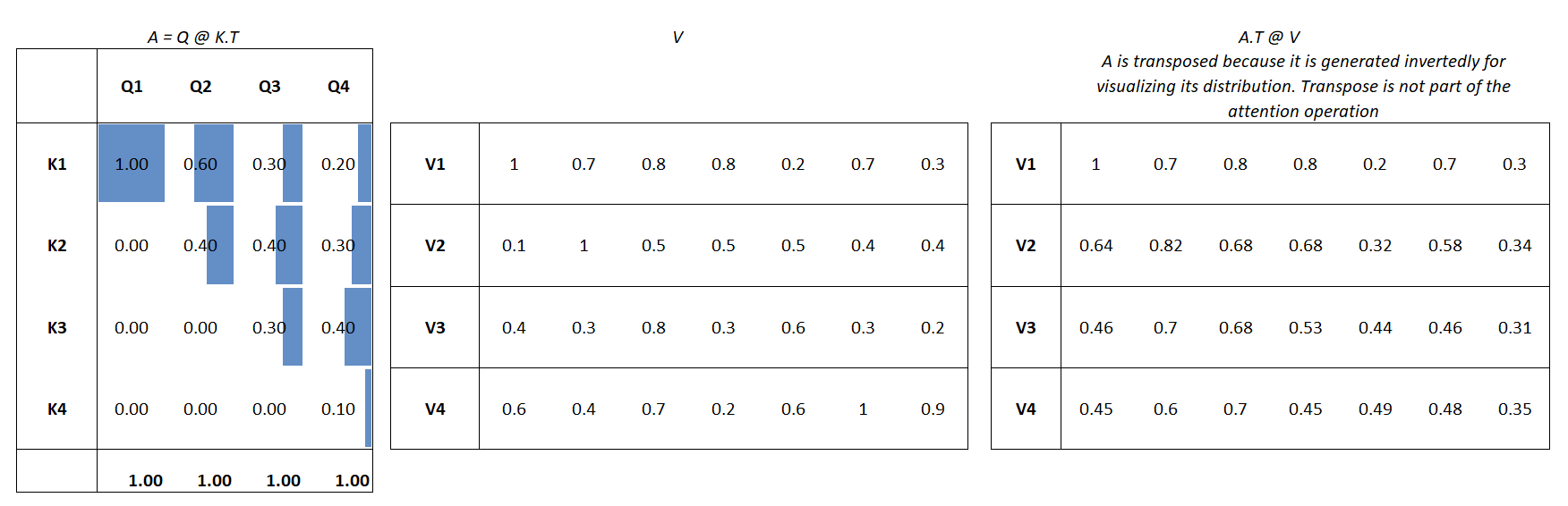
4. We now have an attention pattern A which decides the source and destination of information. The next step can be understood in two different ways: from the point of view of first principles (easy to interpret, discussed in step 5) and from the point of view of computation (used while implementing the computation, discussed in steps 6 and 7).
5. From first principles, you take a weight matrix W_v and use that to project the vectors in the original sequence to the same space as d_model. This project is called V matrix. This modified version of the original sequence of tokens represents the information for each token that will be written to the residual stream if the attention head choses to attend to that token. The next step is to multiply the attention pattern to the V matrix to determine the net change to the embeddings for all tokens in the sequence.

6. In practical implementation, you compute a value vector for each token by projecting the original token to a smaller space. Each weight (from step 3) is then multiplied by the corresponding value vector of that token, and the results are summed to produce a final weighted-average value vector for each token.

   

   Download File here.

7. We now obtain a matrix (d_head * sequence) for each head. Here d_head is the lower dimensional subspace. The matrices (d_head * sequence) are concatenated to form a final matrix (d_model * sequence) [where d_head = d_model / num_heads]. This concatenated matrix is multiplied by a learnable output matrix (d_model * d_model), and the result is added to the residual stream. This variation is mathematically equivalent but computationally more efficient.

Although concatenation and multiplication provide computational efficiency, conceptually, it’s best to view each attention head as individually adding its results to the residual stream.

It can be helpful to consider each attention head as operating on its own subspace of the residual stream, reading from and writing back to specific dimensions within it.

Since attention heads facilitate information transfer across tokens, if an attention head appears to attend to a particular token (while other activations are sparse), we cannot necessarily infer much, as models sometimes consolidate contextual information into a single token to be used in later layers.

Because attention heads primarily move information that is already in the residual stream, experiments analyzing circuits through attention heads alone are best suited for tasks where factual recall by the model is not expected. It remains to be explored whether factual recall happens within MLP layers.

Insights on Attention Mechanisms and Circuits

• Attention heads can be conceptually compared to a 1-D convolution: both enable a model to assess long-range dependencies between tokens, though attention supports longer dependencies. Essentially, both serve to transfer context between tokens.

QK and OV Circuits in Attention Mechanisms

1. QK Circuit: Determines the source (keys) and destination (query) of information by identifying the tokens with relevant information for each target token.
2. OV Circuit: Manages the content to be moved between tokens.

Analyzing attention behavior is more intuitive when viewing QK and OV circuits as separate units rather than focusing on individual Q, K, V vectors.

• QK Circuit: This generates a probability distribution.
• OV Circuit: Retrieves useful information from the residual stream, representing the source and destination of information.

The multiplication of these two circuits facilitates information flow across tokens within the context window (sequence).

Circuit Weights:

• QK Circuit: Defined by matrices ( W_q ) and ( W_k ), which represent low-rank approximations. The combined QK circuit (given by ( W_{qk} )) has dimensions (d_model, d_model).
• OV Circuit: Defined by matrices ( W_v ) and ( W_o ), also as low-rank approximations. The combined OV circuit (given by ( W_{ov} )) also has dimensions (d_model, d_model).

Although the QK and OV circuits share dimensions, they perform fundamentally different tasks:

• QK Circuit: Takes embeddings from the residual stream and outputs a scalar representing the pairwise dot product of different vectors.
• OV Circuit: Processes the embeddings from the residual stream and outputs modified vectors corresponding to the inputs it received.

References

1. Neel’s Walkthrough of the Paper
2. A Mathematical Framework for Transformer Circuits